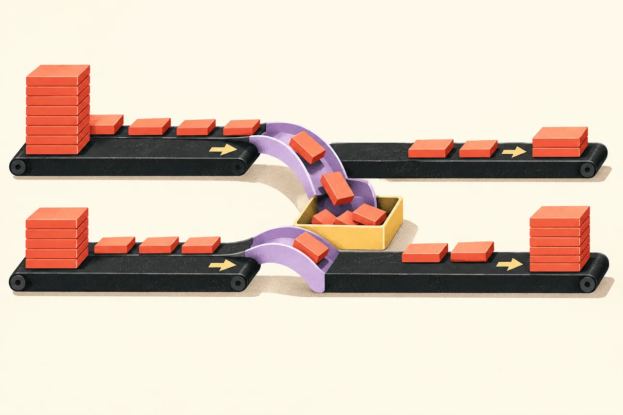
A checkout experiment can generate more orders and more revenue on purchase day, then give back the advantage through refunds. The early report was not necessarily wrong. It may have answered a narrower question than the decision required.
If the team wants to know how much merchandise revenue remains after returns, it needs a refund observation period and a way to connect each reversal to the original order. Comparing one arm’s mature orders with the other arm’s recent orders can distort that answer.
The following example isolates this issue. It concerns reversals after purchase, not how long visitors take to make their first purchase.
Define the revenue measure before reading the result
For this guide, net merchandise revenue means recorded merchandise purchase value minus linked merchandise refunds through a stated follow-up age. It excludes tax, shipping, product costs, payment fees, acquisition costs and future orders.
That definition is useful for a limited comparison. It is not profit, contribution margin or lifetime value. If the decision depends on those measures, the analysis needs the corresponding costs and a separate, explicit calculation.
Keep the original purchase amount and the later refund as distinct records. Google’s ecommerce guide describes refund events that reference the relevant transaction ID and include item information for item-level refund reporting. The order-to-refund connection is also the essential join for an experiment ledger.
Do not assign the refund to whichever experiment version the customer sees when returning an item. The commercial outcome belongs with the original purchase and the assignment used for that comparison.
A result that reverses as refunds arrive
This is a synthetic example with 100 assigned visitors in each arm. Each purchaser places one order on day zero. Everyone has the same observation age, all amounts are US dollars, and there are no further purchases.
Control A produces four $100 orders. Treatment B produces five $90 orders. On day one, neither arm has received a refund.
| Day-one measure | Control A | Treatment B |
|---|---|---|
| Assigned visitors | 100 | 100 |
| Orders | 4 | 5 |
| Purchase conversion | 4% | 5% |
| Gross merchandise revenue | $400 | $450 |
| Revenue per assigned visitor | $4.00 | $4.50 |
Treatment has one additional order and 12.5% more gross merchandise revenue. These tiny counts are for illustration; they do not establish a statistically reliable treatment effect.
Now add the complete fictional refund ledger:
| Original order | Arm | Refund age | Refund amount |
|---|---|---|---|
| A1 | Control | Day 5 | $20 |
| A2 | Control | Day 20 | $30 |
| B1 | Treatment | Day 10 | $90 |
| B2 | Treatment | Day 25 | $90 |
At day 30, control has $50 in refunds and treatment has $180. The two control refunds are partial; the two treatment refunds reverse those orders’ full merchandise amounts.
| Day-30 measure | Control A | Treatment B |
|---|---|---|
| Original gross revenue | $400 | $450 |
| Merchandise refunds | $50 | $180 |
| Net merchandise revenue | $350 | $270 |
| Net revenue per assigned visitor | $3.50 | $2.70 |
Treatment’s net revenue per visitor is now approximately 22.9% lower. The arithmetic is (2.70 − 3.50) / 3.50. The order-conversion metric still records five original purchasers versus four; it has not become the net-revenue metric merely because refunds arrived.
Keep the denominator attached to the decision
Revenue per assigned visitor includes people who never purchased. That makes the denominator consistent with a visitor-level checkout experiment and captures both purchase likelihood and the revenue that remains.
Dividing only by purchasers answers a different question. In this example, the treatment creates more purchasers but retains less revenue per assigned visitor after refunds. A purchaser-only calculation would hide part of the commercial tradeoff by conditioning on an outcome the checkout may affect.
If your experiment randomizes a different unit, define the corresponding analysis carefully. An order-level experiment and a visitor-level experiment do not automatically share the same denominator. Returning customers and multiple orders need rules established before the readout.
Keep these definitions in the metric specification: assignment unit, qualifying order status, included monetary components, refund linkage, follow-up clock and treatment of repeat orders.
Compare orders at a common age
The example is deliberately simple because every order occurs on day zero. Real experiments usually enroll people and collect orders across many days. At a fixed reporting date, older orders have had more opportunity to generate refunds.
Choose the observation rule in advance. One approach is to report revenue for a defined purchase cohort after every included order has reached the required refund age. Another is to define a visitor-level window that includes purchases and reversals under a fully specified timing rule. Those approaches answer different questions; do not combine them silently.
Show the amount of immature revenue separately. If recent orders have not completed the observation period, label the readout accordingly rather than treating missing future refunds as confirmed zero refunds.
The right horizon depends on the business’s return policy and actual processing delays. A 30-day horizon here is a teaching choice, not a recommended universal waiting period. Late reversals beyond the chosen horizon remain outside the measure and should be acknowledged.
Make the refund ledger auditable
Each refund record should identify the original order, its own unique refund identity, timestamp, currency and amount. Preserve partial refunds as separate adjustments so the team can reconcile multiple reversals without overwriting the order history.
Check that repeated notifications do not create repeated deductions. Flag cumulative merchandise refunds exceeding the relevant original merchandise amount for investigation. Exchanges, store credit, canceled orders and chargebacks may require different treatment; define their inclusion rather than assuming every reversal is the same event.
Google’s refund event reference specifies a transaction ID and separates merchandise value from tax and shipping. If the warehouse’s commercial definition differs from the analytics event, document that difference before comparing totals.
Present the early and mature views together
A useful readout can show purchase conversion, gross revenue, refunds, net revenue and cohort maturity side by side. The early view explains what the checkout initially produced. The mature view shows what remained within the agreed horizon.
Then investigate why the patterns differ. More refunds could reflect product mix, misleading expectations, operational problems or random variation. The ledger establishes the amount and timing; it does not identify the cause by itself.
Make the release decision using the preselected commercial measure and an appropriate uncertainty analysis. The synthetic example does not justify stopping a real experiment after a few refunds. It demonstrates why celebrating purchase-day revenue alone can leave a material part of the result unread.